| Stress - Strain | |
|
| Flexure Equation | 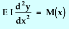 |
|
| Deflection of Rod at Center | 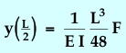 |
|
| Moment of Inertia (circular cross-section) |  |
|
| Frequency of Oscillation | 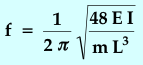 |
PRELAB
PURPOSE
To measure the Modulus of Elasticity (Young's Modulus) using the vibrating loaded rod technique. Several materials will be examined and the Moduli compared.
EQUIPMENT Vernier DataLogger timer, photogate, several 1/4 in diameter solid rods of various materials, mass holder with masses.
RELEVANT EQUATIONS
| Stress - Strain | |
|
| Flexure Equation | |
|
| Deflection of Rod at Center | |
|
| Moment of Inertia (circular cross-section) | |
|
| Frequency of Oscillation | |
DISCUSSION
The amount of flexure y(x), of a uniform rod depends on the Young's modulus of the material from which the rod is constructed.
Fig. 18.1: A Long Thin Rod under Flexure
As shown in Figure 18.1, we will consider a very simple situation, where a mass m is suspended from the middle of the rod causing it to deflect from its normal shape. If the mass is much greater than that of the rod itself, we can neglect the deflection caused by the rod's own mass. Of course the mass must not be so large that the deflection exceeds the elastic limit of the material. An interesting but easy way to measure the Modulus is to set the rod with the mass load into oscillation and to measure the frequency. The derivation of the relationship between frequency and the Young's Modulus of the rod material is somewhat involved, but is not difficult to follow.
We need to obtain the flexure function y(x) that results from loading a rod in the middle. The general equation that governs this type of calculation is called the flexure equation (derived, for instance, in engineering texts on strength of materials).
|
|
(1) |
Equation (1) shows that the second derivative of the flexure y(x) with respect to horizontal distance x is related to the moment, M(x), that results from the loading applied to the rod. The coefficients in this equation are the Elastic (Young's) Modulus E, and the moment of inertia of the cross-section I. We will deal with the latter quantity later. Figure 18.2 shows the force diagram for a mass suspended from the center of the rod. The force is the weight of the mass, and is given by F = m g.
Fig: 18.2: Force Diagram of a Centrally Loaded Rod
Note that the condition for equilibrium requires that both supports provide exactly one-half the applied force in the upward direction. The moment function M(x), can be derived by using the following reasoning. Suppose we make an imaginary "cut" in the rod at position x. We retain all of the rod to the right of the cut, but discard the part of it that lies to the left of the cut and replace it with sufficient torques (moments) to maintain the equilibrium condition.

Fig 18.3: Construction for Determination of the Moment Function
This can be done by adding equal but opposite pairs of forces at the cut point x. The pairs add no net force, but they do affect the torques. A diagram of this procedure is shown in Figure 18.3. The force supplied by the right-hand support, F/2 upward, is duplicated at location x, and an equal but opposite force F/2 downward is added. The downward force at x and the upward force at the right end form a "couple" that applies a torque or moment equal to F/2 times the distance between them, which is L - x in this case if we assume the rod has length L between supports. In a similar fashion, the middle applied downward force F is paired with an upward force of the same magnitude at x. The moment from this couple is F (L/2 - x). We can therefore write down the moment function by adding these two contributions:
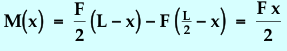 |
(2) |
The next step is to integrate the flexure
equation twice to obtain y(x). The constants of integration are
obtained from the boundary conditions on the derivative at the middle
(![]() )
and on the function itself at the support points:
)
and on the function itself at the support points:
![]() .
You can show that the flexure as a function of position along the rod is
given by:
.
You can show that the flexure as a function of position along the rod is
given by:
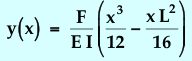
However, since we are interested only in what happens at the center of the rod, we need only to evaluate the flexure at the center:
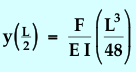 |
(3) |
We model the oscillating rod as a simple
harmonic oscillator with a mass m suspended on a spring of spring
constant k. In that case the frequency of oscillation is
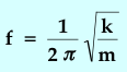 .
In the case of the rod, we know the mass but what about the "spring constant"?
Look at the basic definition of k as the ratio of the applied force
to the deflection it produces. In other words, for the rod we want to take
the ratio of the applied force F to the flexure where it is applied,
.
In the case of the rod, we know the mass but what about the "spring constant"?
Look at the basic definition of k as the ratio of the applied force
to the deflection it produces. In other words, for the rod we want to take
the ratio of the applied force F to the flexure where it is applied,
![]() .
The resulting expression for the frequency of oscillation for a uniform
rod of length L that is loaded at the center by a mass m
is thus:
.
The resulting expression for the frequency of oscillation for a uniform
rod of length L that is loaded at the center by a mass m
is thus:
|
|
(4) |
The only remaining quantity that we need to evaluate is I, the moment of inertia with unit density of the cross-section about its midline. By definition it is given by:
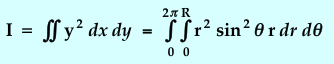
where R is the radius of the circular cross-section, as shown in Figure 18.4.
Fig. 18.4: Set-up for Calculation of Moment of Inertia
The indicated integration is switched
from Cartesian to Polar coordinates by substituting for the differential
area element dx dy = r dr dθ,
and for the coordinate y = r sinθ.
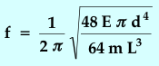
The integration is straight forward and the resulting moment of inertia
is:  . The
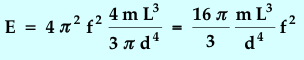
final expression for the frequency of oscillation in terms of the diameter
of the rod is therefore:
. The
final expression for the frequency of oscillation in terms of the diameter
of the rod is therefore:
 |
(5) |
and Young's Modulus can be obtained from careful measurements of the frequency from the formula:
 |
(6) |
Print out and complete the
Prelab questions.